Relation between standard deviations of population and sample learned from numerical experiment.
A textbook formula for standard deviation of sample is wrong. The correct version of standard deviation of the sample is derived from series of numerical experiments and presented in the article.
Standard deviation is one of the most basic characteristics of any statistical analysis of experimental data. It has sense of average deviations from average value in series of measurements.
Formulas for calculation of standard deviation look like trivial until thoughtful person would notice that there are at least two of them. One is for standard deviation of population of size n:
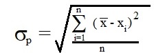
|
(1) |
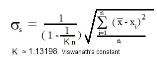
and other for standard deviation of sample of size n from population of any size (?):
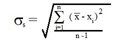
|
(2) |
where x - average value of all measurements calculated by formula:
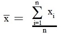
|
(3) |
Standard deviation of sample can be interpreted as average distance of all measurements from their mean (average). It is in normal language a measure of expected consistency in a row of measurements. The important moment is that dispersion of the numbers in series can have two different reasons. First of them is nature of the experimental parameter. It can have dispersion of the measured property by fact of its nature. Or a measurement process can have (and in fact always has) limitation in precision, for example in establishing an exact numerical value of physical constants from indirect experiments.
As one can see that formulas 1 and 2 for standard deviations of population and sample correspondingly are almost identical except that for whole population averaging is done for all measurements and for sample for all but one. The justification for formula 2 is the assumption that average dispersion (calculated by formula 1) of subset of population will be less then dispersion for all population thus formula must be corrected to reflect dispersion of whole population that one should be interested in (no necessary as will be shown later).
It is confusing. Is really true that formula 2 for standard deviation of sample gives on long run the value of standard deviation of population? It is clear correct when big size of populations and size of sample is approaching to size of population ns → np both standard deviations are the same σs → σp . But what is about for small sample when ns <≈ 20? The practically relevant question for me is formulated in following way:
What is relation between statistics of sample of population and statistics of population as a whole? The direct and transparent way to answer is numerical simulation experiment.
Formulation of the problem. There is a city with population of N people. The firm has contract to research its demographic. It hires Nagents each of them polls Ns distinct persons, where Ns is the size of sample. Upon privacy concerns agents report their findings in general form as mean (average) and average dispersion (calculated by formula 1) of characteristics like age in sample. The problem is to learn what relation between results of such research and actual demographic of the city.
Numerical experiment procedure.
Step 1. Building sample of demographic.
Creating and randomly filling up the array A[N] with size N that represent an actual demographic of city population. Here and later, for specificity sake, we will be talking about one characteristic - age. But findings of the numerical experiments can be applied to any measurable characteristic (income, education and so on). The influence of specific distribution of age in population on the relation with output of numerical experiment has to be one of the finding.
Step 2. Repeat Nagents times a procedure of selection Ns distinct and random by index points in A[Ns] array and store them in S[Ns] array (sample). Calculate average (formula 3) and standard dispersion (formula 1) for each A[Ns] and S[Ns] array - Ais and Sis.
Step. 3 Repeat Step 2 for, different sizes of sample, Ns.
Step. 4 Compare statistical characteristics for different sizes of sample between each other and with statistical characteristics of whole population.
Step 5. Repeat steps above for different demographics by its statistical distribution and make conclusions.
Big size experiment.
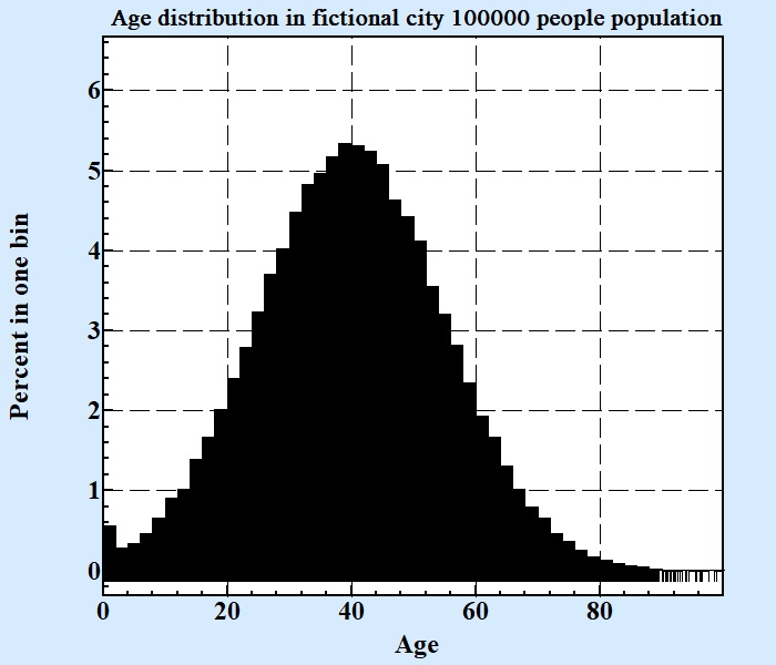
To be convinced about validity of findings the first numerical experiment will be performed with really big size population: 100000. The histograms of the age distribution that is constructed to be with average 40 and standard deviation 15 (all positive) is presented at Fig 1
We did 1000 selections with different sizes of sample by 1000 fictional agents for each of sample size. At Fig. 2 distribution of averages and standard deviations for different samples are shown:
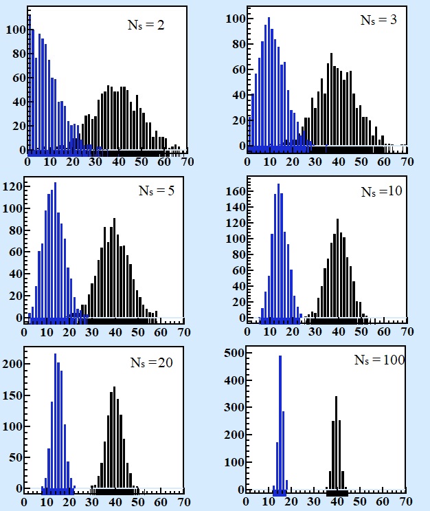
As it should be expected the larger size of sample the less dispersion both average and standard deviations of sample. What is qualitatively differ between average sample and standard deviation of sample is that maximum of distribution of average coincides with average of whole population and its distribution itself is symmetrical around maximum.
Distribution of standard deviation of sample is not symmetrical. Standard deviation by definition has only positive values (or zero). The smaller size of sample the bigger a shift of its maximum position to smaller values and thus there is systematic underestimation of standard deviation of sample calculated by formula 1 compare to actual (natural) value for dispersion of measured property in whole population. Is formula 2 correct this systematic mismatch with actual standard deviation? Or there could be other better formula for calculation of standard deviation of the sample that in average gives the same result as standard deviation of population?
At Fig. 3 there are shown average by Nagents standard deviations calculated for different sizes of sample. The chart displays results only in interval from Ns = 2 till Ns = N where N is size of whole population.
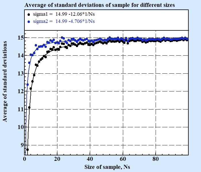
As it can be see from Fig 3 both formulas 1 and 2 give underestimated values of average standard deviation of sample these are in need to be corrected for produce value equal to standard deviation of population.
The following formula produces the correct value of average standard derivation of sample for any Ns:
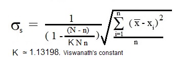
|
(4) |
Formula 4 gives standard deviating for sample with size n = Ns randomly selected from population with size N.
It is important to emphasize that standard deviation of sample is random number by its definition in the contrary to the standard deviation of the population that is constant for given population. Formula 4 returns the value that should be interpreted in following manner: if there is a population with some diverse characteristic its standard deviations will be best fit by average of standard deviations of subset samples of this population calculated by formula 4.
We did numerical numerical experiment to verify correctness of applicability of the formula 4 to estimate standard deviation of population on the base of averages of standard deviations of random samples:
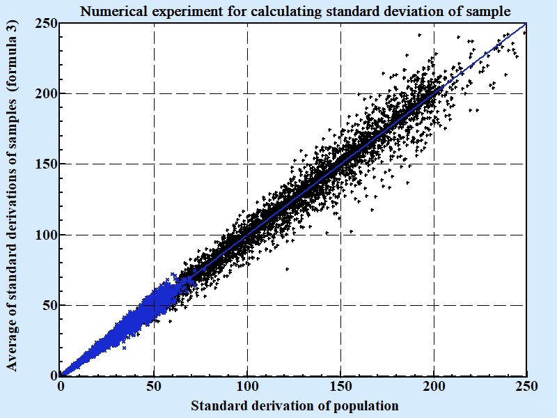
The numerical experiment results of which presented at the Fig.4 was done by following scheme. The random size (from 7 till 100000) population is created and randomly populated by Gaussian like numbers with random mean and standard deviation; other variant of population distribution is uniformly between two random borders. For each population standard deviation calculated and then 100 times samples randomly selected and average of standard deviations, calculated by formula 4, compared with standard deviation of whole population. As it is seen at Fig. 4 they have so strong correlation that one can safely presume their equality.
Formula 4 compare with formulas 2 has fundamental advantage. It is not confusing. In case of formula 2 if populating is reasonable small one can be puzzled why adding one person to the sample and selecting by this the whole population the formula must be switched to formula 1. It sounds sort of arbitrary action. Formula 4 is free from such ambiguities. For N = n formula 4 is exact equal to formula 1 for standard deviation of population. For size of populations when N → ∞ (actually just when N > 100) the formula 4 is transforming to the form:
|
(5) |
The practical significance of applying more precise formula for calculation standard deviation of sample is not so obvious in spite its fundamental role in statistics. It is true that established, standard, formula 2 gives underestimated value of standard deviation. The question is it important enough in practice? Taking into account that standard deviation of sample is a random parameter by itself is it critical for anything to estimate mistake more correctly is important enough to correct wrong formula? I have no idea. Everybody should decide for himself is it worst to bother to be slightly closer to truth on the long run or better to keep using traditional formula no matter that it is systematically presenting underestimated output.
My advise is to be even more skeptical in results of polling. If political poll gives accuracy in 4% it most possible means that mistake is larger... Maybe 6%, maybe 10%. It depends... not on formulas, really.
Apr. 20, 2018; 17:43 EST